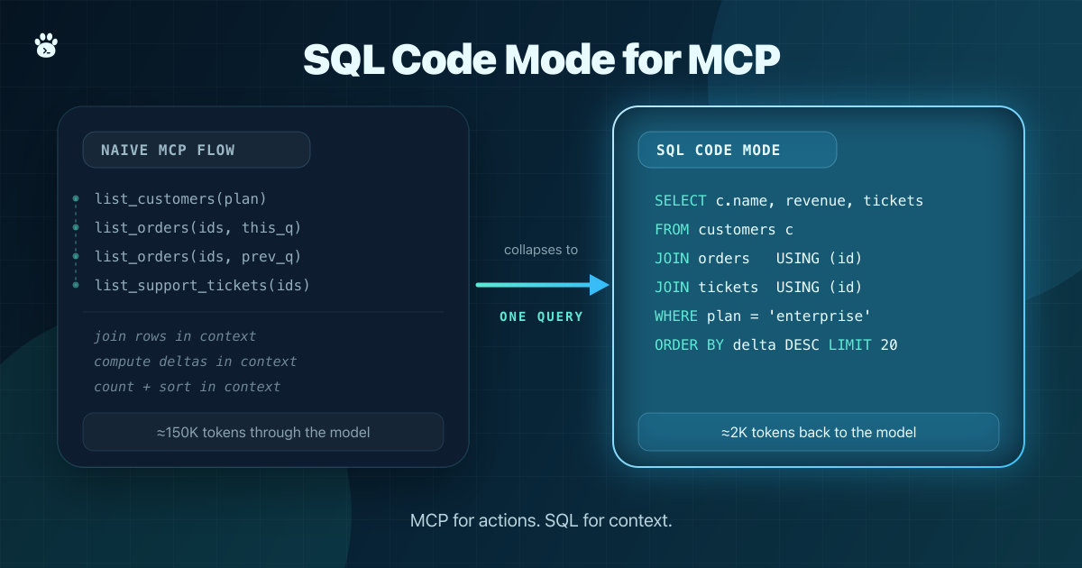
Today, most MCP servers expose one tool per operation, so you end up with tools like get_customers, get_orders_by_customer, get_ticket_counts, search_issues, and list_pull_requests. That works when the user request maps cleanly to one operation, but it breaks down when the question spans across multiple tools.
Then the agent has to run a chain of calls and join the intermediate results in its context window. It fetches customers, then orders, then tickets, then tries to line up IDs, compute totals, filter rows, sort the result, and explain the answer. The slow part is not just the network traffic; it is the join happening in the model context, which is the motivation behind Code Mode.
Instead of asking the model to request every operation one at a time, the server gives it a code-execution tool. The model writes a small program, and that program becomes the plan: call the configured tools, process intermediate results inside the execution environment, and return only the information needed for the final response.
In a good implementation, those configured tools are exposed to the generated code as typed methods. The model can use normal programming constructs like variables, loops, conditionals, maps, and filters instead of stretching the same logic across multiple model-tool turns. Depending on the server, the available methods may be described up front or discovered as the task narrows.
The problem is easiest to see with a normal business question:
Which enterprise customers had declining order revenue this quarter and more than three support tickets in the same period?
There is a query hiding inside that sentence. It has a filter, two time windows, a join, a grouping step, a comparison, and a limit. You can expose five different MCP tools and ask the model to stitch the answer together, but then the model is doing the work a query engine should do.
The naive MCP flow looks something like this:
list_customers(plan = "enterprise")
list_orders(customer_ids = [...], start = ..., end = ...)
list_orders(customer_ids = [...], previous_start = ..., previous_end = ...)
list_support_tickets(customer_ids = [...], start = ..., end = ...)
join customers to orders in context
compute quarterly deltas in context
count tickets in context
sort and format in context
The failure mode is structural: raw records move through the model context, relational logic is implemented by the model, and the analytical plan is buried in a transcript of tool calls.
The SQL version is dull in the useful way:
WITH current_revenue AS (
  SELECT
    customer_id,
    SUM(total_cents) AS current_total_cents
  FROM orders
  WHERE order_date >= DATE '2026-04-01'
    AND order_date <  DATE '2026-07-01'
  GROUP BY customer_id
),
previous_revenue AS (
  SELECT
    customer_id,
    SUM(total_cents) AS previous_total_cents
  FROM orders
  WHERE order_date >= DATE '2026-01-01'
    AND order_date <  DATE '2026-04-01'
  GROUP BY customer_id
),
ticket_counts AS (
  SELECT
    customer_id,
    COUNT(*) AS ticket_count
  FROM support_tickets
  WHERE created_at >= TIMESTAMP '2026-04-01 00:00:00'
    AND created_at <  TIMESTAMP '2026-07-01 00:00:00'
  GROUP BY customer_id
)
SELECT
  c.id,
  c.name,
  current_revenue.current_total_cents,
  previous_revenue.previous_total_cents,
  ticket_counts.ticket_count
FROM customers c
JOIN current_revenue ON current_revenue.customer_id = c.id
JOIN previous_revenue ON previous_revenue.customer_id = c.id
JOIN ticket_counts ON ticket_counts.customer_id = c.id
WHERE c.plan = 'enterprise'
  AND current_revenue.current_total_cents < previous_revenue.previous_total_cents
  AND ticket_counts.ticket_count > 3
ORDER BY
  previous_revenue.previous_total_cents - current_revenue.current_total_cents DESC
LIMIT 20;
In that loop, the model maps the user's question to a query, the query engine handles joins, grouping, comparison, sorting, and row limits, and the model gets back a small result to explain. That's SQL code mode.
Code Mode, but for Data
Anthropic's Code execution with MCP made the general code-mode argument clearly: direct tool calls force tool definitions and intermediate results through the model context. Their example cut a workflow from 150,000 tokens to 2,000 by moving orchestration into an execution environment. Cloudflare's Code Mode applies the same pattern to large APIs by exposing search() and execute() instead of thousands of endpoint-shaped tools.
The point is not "let the model run arbitrary code," a framing that makes the pattern sound more dangerous and less precise than it needs to be. The point is to move deterministic work out of the context window and into an execution engine.
Most production MCP servers sit in front of systems that already have their own execution model: relational databases and warehouses, REST APIs described by OpenAPI, GraphQL APIs, or other MCP servers. MongoDB and Elasticsearch fit too, but SQL, OpenAPI, GraphQL, and MCP composition are enough to make the point.
The common thread is that each backend can carry part of the plan more reliably than the model. Databases handle filters, joins, aggregations, sorting, windows, and projections. REST APIs expose endpoint contracts, pagination, and batching boundaries. GraphQL lets the caller select fields and relationships in one operation instead of walking them through tools.
So code mode should usually follow the backend's native surface:
- SQL pushes joins, aggregations, filters, and window functions into the database or query engine.
- OpenAPI-backed runtimes let the model write a bounded server-side plan that calls a REST surface, handles pagination, and returns a shaped result.
- GraphQL operations select the fields and relationships needed in a single round trip.
- MCP composition runtimes call multiple underlying MCP tools, filter results, and return only the composed output.
The goal is not to make the LLM a better tool-chain orchestrator. It is to stop routing deterministic work through the LLM when the backend can execute it. For an API, the runtime may be JavaScript that calls a typed client, handles pagination, and returns only the fields needed for the answer. For data, the runtime is often SQL, and the pattern is simple:
discover schema -> generate SQL -> validate SQL -> execute SQL -> return capped result
The MCP server might expose tools like search_tables, describe_table, and query. The model still uses MCP, but instead of calling a long sequence of domain-specific tools, it writes a single query against a known surface.
That boundary matters. SQL code mode is not a database shell for the model. The server should parse the SQL, reject unsupported statements, enforce read-only behavior by default, apply timeouts, cap returned rows, and log what ran. The model writes the query, but the server owns the boundary.
DuckDB as the Agent's Scratch Database
The best way to think about DuckDB here is as a scratch database for the agent: a place where file data, API results, and temporary tables can be inspected and joined without pushing raw rows into context. It is embedded, fast enough for real analytical work on local data, and can read CSV, JSON, and Parquet directly.
That changes the agent loop because, instead of loading CSV or JSON directly into context, the agent can ask the runtime what shape the data has:
DESCRIBE SELECT *
FROM read_csv_auto('customers.csv');
Once it knows the columns and types, it can write a query over the data in place:
SELECT
  a.account_name,
  a.owner,
  SUM(o.total_cents) / 100.0 AS revenue
FROM read_csv_auto('accounts.csv') a
JOIN read_parquet('orders/*.parquet') o
  ON o.account_id = a.account_id
WHERE o.order_date >= DATE '2026-01-01'
GROUP BY a.account_name, a.owner
ORDER BY revenue DESC;
If the question requires a trend or a ranking, the agent can reach for normal analytical SQL:
WITH monthly AS (
  SELECT
    account_id,
    date_trunc('month', order_date) AS month,
    SUM(total_cents) AS revenue_cents
  FROM read_parquet('orders/*.parquet')
  GROUP BY account_id, month
),
with_previous AS (
  SELECT
    account_id,
    month,
    revenue_cents,
    lag(revenue_cents) OVER (
      PARTITION BY account_id
      ORDER BY month
    ) AS previous_revenue_cents
  FROM monthly
)
SELECT
  account_id,
  month,
  revenue_cents,
  previous_revenue_cents,
  revenue_cents - previous_revenue_cents AS delta_cents
FROM with_previous
WHERE previous_revenue_cents IS NOT NULL
ORDER BY delta_cents ASC
LIMIT 20;
DuckDB becomes the agent's local workspace: raw data rows live there while the model inspects schema, chooses inputs, writes SQL, and explains the result. Joins, rankings, windows, and arithmetic stay in the database.
A minimal DuckDB-backed MCP server for this pattern does not need many tools. It can start with schema inspection, query execution, and cancellation. The hard parts sit behind those tools: path restrictions, read-only execution, single-statement enforcement, timeouts, row caps, and audit logs.
A Small Version You Can Build
The next step is to bring API data into the same DuckDB session, and you do not need a full platform to prove the idea. A small Python process can call a REST endpoint, normalize the JSON into rows, register those rows as a DuckDB view, and let the agent write SQL against this pipeline:
REST or OpenAPI endpoint -> Python loader -> DataFrame -> DuckDB view -> SQL query
Here is a minimal version of the loader:
import os
import re
from typing import Any

import duckdb
import pandas as pd
import requests

con = duckdb.connect(":memory:")
IDENTIFIER = re.compile(r"^[A-Za-z_][A-Za-z0-9_]*$")


def checked_identifier(name: str) -> str:
    if not IDENTIFIER.fullmatch(name):
        raise ValueError(f"invalid DuckDB identifier: {name}")
    return name


def at_path(value: Any, path: list[str]) -> Any:
    for key in path:
        value = value[key]
    return value


def register_rest_view(
    name: str,
    url: str,
    *,
    headers: dict[str, str] | None = None,
    params: dict[str, str] | None = None,
    result_path: list[str] | None = None,
) -> None:
    name = checked_identifier(name)
    response = requests.get(
        url,
        headers=headers or {},
        params=params or {},
        timeout=30,
    )
    response.raise_for_status()

    data = response.json()
    rows = at_path(data, result_path or [])
    frame = pd.json_normalize(rows)

    con.register(f"{name}_raw", frame)
    con.execute(f"CREATE OR REPLACE TEMP VIEW {name} AS SELECT * FROM {name}_raw")
For a GitHub endpoint, the loader can turn an API response into a queryable view:
register_rest_view(
    "github_pulls",
    "https://api.github.com/repos/CITGuru/pawrly/pulls",
    headers={"Authorization": f"Bearer {os.environ['GITHUB_TOKEN']}"},
    params={"state": "open", "per_page": "100"},
)
The agent does not need the raw JSON response because it can inspect the view:
DESCRIBE github_pulls;
Then query the API result with normal SQL:
SELECT
  "user.login" AS author,
  COUNT(*) AS open_prs
FROM github_pulls
GROUP BY author
ORDER BY open_prs DESC;
For OpenAPI, the same idea can be driven from the spec. The minimal version is just enough to find a GET operation, substitute path parameters, pass query parameters, and register the returned collection as a view:
def find_operation(spec: dict[str, Any], operation_id: str) -> tuple[str, dict[str, Any]]:
    for path, methods in spec["paths"].items():
        for method, operation in methods.items():
            if method.lower() == "get" and operation.get("operationId") == operation_id:
                return path, operation
    raise KeyError(f"GET operation not found: {operation_id}")


def register_openapi_view(
    name: str,
    spec: dict[str, Any],
    operation_id: str,
    *,
    base_url: str,
    path_params: dict[str, str] | None = None,
    query: dict[str, str] | None = None,
    headers: dict[str, str] | None = None,
    result_path: list[str] | None = None,
) -> None:
    path, _operation = find_operation(spec, operation_id)

    for key, value in (path_params or {}).items():
        path = path.replace("{" + key + "}", value)

    register_rest_view(
        name,
        base_url.rstrip("/") + path,
        headers=headers,
        params=query,
        result_path=result_path,
    )
This is not a production OpenAPI engine; it skips auth schemes, pagination styles, schema references, rate limits, retry policy, nested response shapes, and safety rules. But it demonstrates the core move: the API call is not the final interface; the API call populates a relation, and the agent works against the relation.
Once the data is in DuckDB, the agent can join API data with local files:
SELECT
  a.account_name,
  COUNT(p.number) AS open_prs
FROM read_csv_auto('accounts.csv') a
JOIN github_pulls p
  ON p."user.login" = a.github_login
GROUP BY a.account_name
ORDER BY open_prs DESC;
The prototype exposes both the mechanics and the chores. Once the pattern works, you have to deal with pagination, credentials, schema drift, required filters, caching, source-specific safety limits, and whether a field should be joinable but not returned to the model. That is where the Python bridge starts turning into a source layer.
The Data Stops Being Local
Real agent data workflows rarely stay inside one DuckDB session. The useful context can be spread across GitHub issues, Linear tickets, Stripe invoices, Postgres tables, S3 objects, Slack exports, internal REST APIs, and other MCP servers, and each source brings its own structure: OAuth, pagination, required filters, rate limits, caching, and business definitions that should not be reinvented in every prompt.
At that point, SQL mode needs more than an embedded engine. It needs a catalog and a source layer that can answer questions like:
Which tables exist?
Which columns can I filter on?
Which filters are required?
Which predicates can be pushed into the API?
Which source owns authentication?
Which result should be cached?
Which query should be refused before it scans?
That is the jump from a local scratch database to a query workspace for agents.
From Scratch Database to Source Layer
One way to run SQL across sources is to put a query layer in front of the systems an agent would otherwise reach through separate tools. At that point, a single DuckDB connection with simple views is no longer enough. We need a layer that exposes catalog where files, object storage, REST and GraphQL APIs, OpenAPI-described services, databases, warehouses, lakehouse tables, and external MCP servers can all be described as queryable inputs.
This does not replace MCP. The agent can still connect through MCP, but the read path changes from receiving a large set of unrelated tools to inspecting a catalog and submitting a query.
Pawrly is one implementation of that source-layer approach: a query engine that gives agents a SQL interface over systems they usually reach through separate tools, including REST and GraphQL APIs, files, databases, and MCP servers. It keeps the agent-facing interface as SQL while an isolated workspace owns source definitions, credentials, pushdown rules, and caching behavior.
For example, in Pawrly that workspace is declared in pawrly.yaml. Each source becomes a SQL schema. HTTP sources can push SQL filters into path, query, or body parameters. MCP sources can expose read operations from another MCP server as SQL tables or table-valued functions. Files and databases share the same query surface. Caching and materialization are explicit instead of hidden in generated scripts.
A minimal workspace might start with local files:
version: 1
name: sql-mode-demo

sources:
  - name: data
    kind: file
    tables:
      - name: accounts
        path: ./data/accounts.csv
        format: csv
      - name: orders
        path: ./data/orders.parquet
        format: parquet
Then it can add an API source:
sources:
  - name: github
    kind: http
    config:
      base_url: https://api.github.com
      token: ${secret:GITHUB_TOKEN}
    tables:
      - name: pulls
        endpoint: /repos/{owner}/{repo}/pulls
        params:
          - { name: owner, required: true }
          - { name: repo, required: true }
          - { name: state, default: open }
        response:
          path: $
          schema:
            - { name: number, type: bigint }
            - { name: title, type: varchar }
            - { name: state, type: varchar }
            - { name: user_login, type: varchar, source: $.user.login }
Once those sources exist, the agent does not need separate "get accounts," "get orders," and "list GitHub pull requests" tools for every analytical question. It can ask for schema context and run a query:
SELECT
  a.account_name,
  SUM(o.total_cents) / 100.0 AS revenue,
  COUNT(p.number) AS open_prs
FROM data.accounts a
JOIN data.orders o
  ON o.account_id = a.account_id
LEFT JOIN github.pulls p
  ON p.user_login = a.github_login
WHERE p.owner = 'CITGuru'
  AND p.repo = 'pawrly'
  AND p.state = 'open'
GROUP BY a.account_name
ORDER BY revenue DESC
LIMIT 50;
That query is not meant to be a perfect business metric. It shows the interface: the agent writes SQL over sources that do not naturally live in the same system. The query layer handles source access, pushdown, execution, and result shaping, then returns a bounded result.
For common business questions, a semantic layer can sit on top of the raw tables. That matters because "revenue," "active customer," and "open engineering work" are not just column names. They are definitions. Raw SQL is useful for exploration, but repeated agent workflows need measures, dimensions, relationships, required filters, and row-level rules that live outside the prompt.
The Safety Contract
SQL code mode is only useful if the execution boundary is explicit. The model should not be trusted because it produced plausible SQL, so the server has to enforce the contract by starting read-only and adding controls in layers:
Parse the SQL.
Reject unsupported statement types.
Require a single statement.
Resolve referenced tables and functions.
Check source-level safety rules.
Push filters down where possible.
Apply a timeout.
Apply max rows and response-size caps.
Record the query, caller, sources, row count, and truncation flag.
For API-backed tables, safety is not only about SQL syntax. A query can be read-only and still be dangerous if it fans out across thousands of API calls. The source layer needs its own controls: required filters, maximum pages, default limits, timeouts, and cache policies. For sensitive domains, the server should distinguish fields that can be used for joins from fields that can appear in output.
The model can be told to write safe SQL, but the server still has to prove the SQL is safe before it runs. That proof comes from parsing, policy checks, least-privilege credentials, and execution limits, not from a sentence in the prompt.
MCP for Actions, SQL for Context
SQL code mode does not replace MCP tools. It keeps read-heavy work from turning into a long chain of tool calls and intermediate results.
Keep curated tools for actions like creating issues, sending messages, updating records, and triggering workflows. SQL code mode is for long-tail analytical reads where the request is really a query plan.
DuckDB is the right starting point because it shows the pattern with almost no infrastructure. Pawrly shows what changes when the data stops being local: the agent still writes SQL, but the server owns the catalog, credentials, source rules, execution limits, and result shape.